Invariant and Equivariant Classical and Quantum Graph Neural Networks
2023 Google Summer of Code (GSOC) Project under the Organization Machine Learning for Science (ML4SCI) with the Quantum Machine Learning for High Energy Physics team (QMLHEP)
Introduction
Machine learning algorithms are heavily relied on to understand the data generated at the European Council for Nuclear Research’s (CERN) Large Hadron Collider (LHC) which produces immense amounts of data through the measurement of the products of particle collisions. Since data from these events can typically be formed into a graph structure, deep geometric methods, such as graph neural networks (GNNs), have been used as an approach to various HEP anlysis tasks. One such task is jet tagging, where jets are viewed as point clouds with distinct features and edge connections between their constituent particles. To enhance the validity and robustness of deep networks, embedded symmetries, which are present in many physically realizable datasets and fundamental physical theories, can also be discovered by the model through the use of invariant \(I(n)\) and equivariant networks \(E(n)\). However, due to the increasing size and complexity of these datasets, as well as the models which process them, an involved yet computationally inexpensive approach must be utilized. To handle an increase in the complexity of the data, I suggest the implementation of a classical attention (AT) transformer with the necessary modifications to incorporate, invariant or equivariant, and GNN layers. As the extension of classical algorithms via bit-wise processes to quantum algorithms via qubit-wise processes has been rapidly developing over the last few years, I propose the full development of general quantum and equivariant quantum graph neural network (QGNN/EQGNN) architectures to meet the demands of requiring these machine learning algorithms to offer enhanced robustness through the adherence to fundamental physical principles while reducing their computational cost.
Graph Data
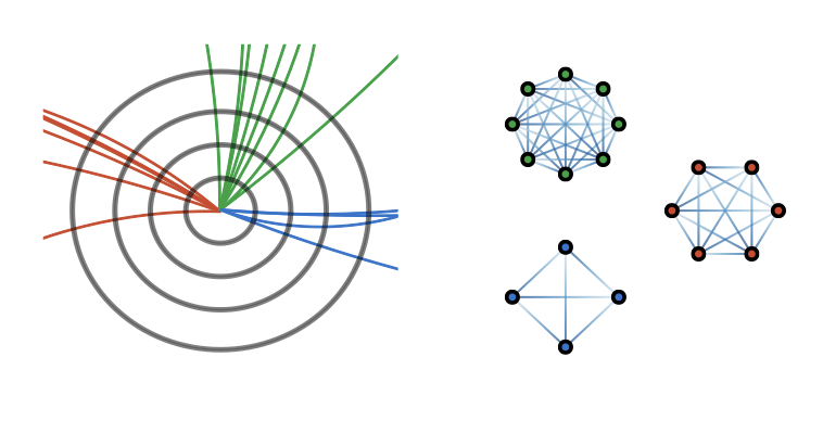
The LHC produces immense amounts of data through the measurement of the products of particle collisions which can be analyzed using various supervised and unsupervised machine learning methods. An example of one important task is jet tagging, which seeks to characterize the particle origin of jets through collections of final-state measurements. By viewing individual jets as point clouds with distinct features and edge connections between the constituent particles which make them up, a graph neural network (GNN) has been considered as a well-suited architecture for jet tagging, as depicted below. A graph \(\mathcal{G}\) is typically defined as a set of nodes \(\mathcal{V}\) and edges \(\mathcal{E}\), i.e. \(\mathcal{G} = \{ \mathcal{V}, \mathcal{E} \}\).
It should be noted that although the visualization displays the same number of nodes m per graph, this number can vary while the number of features per node typically remains constant. In a typical jet dataset, the features per node include the transverse momentum \(p_T\), rapidity \(\eta\), azimuthal angle \(\phi\), and particle ID or particle mass in order to characterize the particle measured in that multiplicity bin. Edge features \(a_{ij}\) can be defined using the features between two nodes. A binary classification task was performed with this dataset to classify whether a jet originated from a quark or a gluon.
Models
The four architectures developed and presented below include classical graph neural networks (GNN) and equivariant graph neural networks (EGNN), as well as, quantum graph neural networks (QGNN) and equivariant quantum graph neural networks (EQGNN).
Invariance and Equivariance
By making a network invariant and equivariant to particular symmetries within a dataset, a more robust general architecture can be developed. In order to introduce invariance and equivariance to the input embeddings or the model architecture, one must assume or learn a certain symmetry which is present within a dataset. This will determine the group \(G\) which defines the symmetry group the dataset is invariant or equivariant under transformations of. Invariance performs better as an input embedding. A function \(f\) is \(\textbf{invariant}\) with respect to a group transformation \(g \in G\), if
\begin{equation} \label{eq:invariance} f(gx) = f(x) \end{equation}
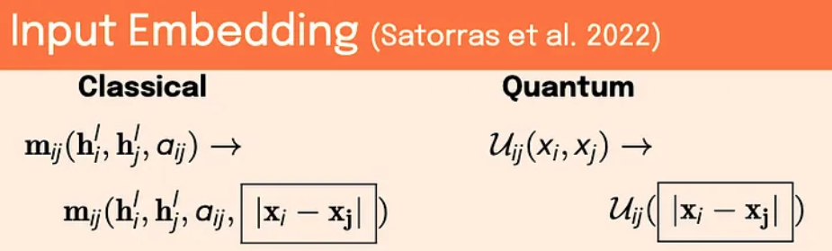
where \(x\) is the input to the model. For example, if a model classifies one jet structure as originating from a quark, and one wants to classify the same jet but now with the nodes rotated in \(\phi\) and \(\eta\) space, the invariant measure would be the distance between nodal coordinates \(|\Delta\phi^2 + \Delta\eta^2|\), rather than the raw coordinates themselves. One can use this distance as the input to a layer rather than the raw coordinates.
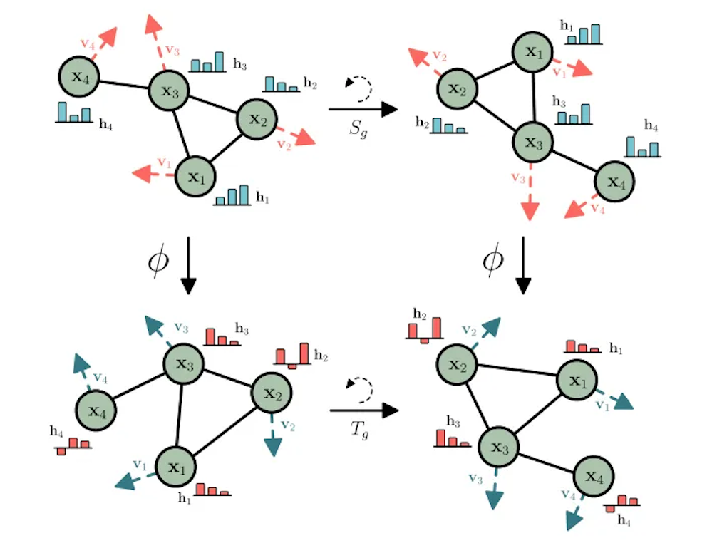
\(\textbf{Equivariance}\) can be more easily incorporated into the model layers. This has been done using simple nontrivial equivariant functions along with higher order methods involving the use of spherical harmonics to embed the equivariance within the network. The approach used here was the simple one and informed by the successful implementation of SE(3), or rotational, translational, and permutational, equivariance on dynamical systems and the QM9 molecular dataset
A function \(f\)$ is equivariant with respect to a group \(G\) transformation \(g \in G\) if
\begin{equation} \label{eq:equivariance} f(gx) = g’ f(x) \end{equation} where \(g : x \to x'\), \(g' : f \to f'\), and \(g \cong g'\).
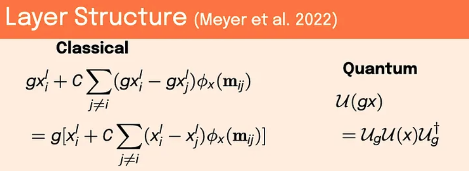
For example, classically, we can consider a data point with coordinates x and its rotated and translated counterpart \(x’ = Qx + T\), where \(Q\) is a rotation matrix and \(T\) is a translational matrix. The rotation \(Q\) and translation \(T\) together define our transformation here, where the group \(Q\) acts under multiplication against the vector space of the data coordinates and \(T\) acts under addition against the vector space of the data coordinates, i.e. \(TQx = Qx + T\). Then, the function \(f(x) = x_i + C \sum_{j\neq i} (x_i — x_j)\), where \(i\) is the nodal index of the graph, becomes equivariant to these transformations of the data. This can be shown by writing
\begin{equation} \label{eq:equivariance_proof} f(gx) = (Qx_i +T) + C \sum_{j\neq i} (Qx_i + T — Qx_j - T) = Q[ x_i+ C \sum_{j \neq i} (x_i — x_j) ] + T = g’ f(x) \notag \end{equation}
Therefore, applying this function to the nodes of a graph and its neighbors allows for equivariance to be implemented naturally within the network. Quantum mechanically, one needs to form a network with operators which commute with the final observable chosen for the final measurement results. Permutation equivariance can also be achieved in the quantum network through classical aggregation methods of the final quantum states A comparison between the classical and quantum formulations can be seen below.
Graph neural network
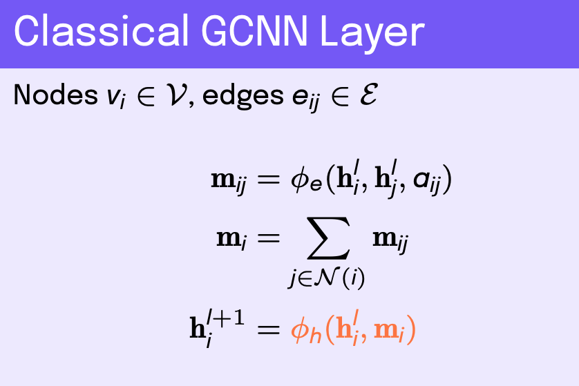
When to exploit the capabilities of graph neural networks (GNNs) depends on the structure of the dataset given. Here, since particle jets are structured to be considered as point clouds, or graphs with well defined nodes and edges, it is appropriate to make use of this network architecture. Classical GNNs take in a collection of graphs \(\{ \mathcal{G}_k \}\) each with nodes \(v_i \in \mathcal{V}\) and edges \(e_{ij} \in \mathcal{E}\) where \(\mathcal{G}_k = \{\mathcal{V}, \mathcal{E} \}\). Each node in the graph has a feature vector \(\mathbf{h}_i\), and the entire graph has an associated edge attribute tensor \(a_{ijr}\) describing relationships between node \(i\) and its neighbors \(j\), where we can define \(N(i)\) as the set of neighbors of node \(v_i\). The edge attribute tensor is just a matrix in the case of one edge feature per node-neighbor pair. These edge attributes are typically formed from the features corresponding to each node and its neighbors.
In the layer structure of a GNN, multilayer perceptions (MLP), or fully-connected NN layers, are used to update the edge attributes as well as the nodal features before aggregating the updated nodal features, typically with an average sum-pooling method, for each graph to form a final classification for each graph
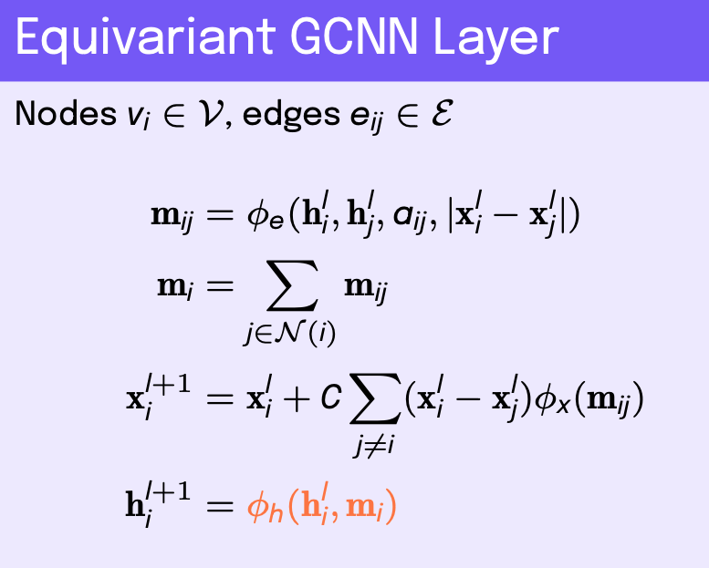
SE(2) Equivariant graph neural network
The SE(2) equivariant graph neural network (EGNN) architecture is similar to that of the GNN, however, an equivariant coordinate update function is introduced at each layer. The invariant distance between these transformed coordinates is then added to the edge MLP, along with its other previously defined inputs. This pattern is illustrated below.
Quantum graph neural network
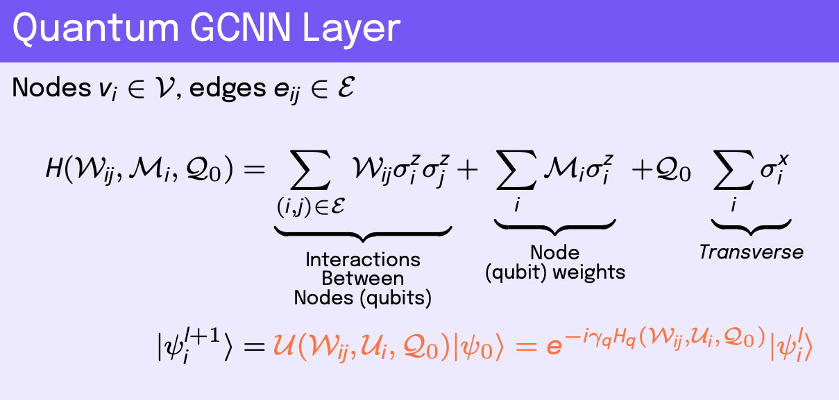
For a quantum GNN (QGNN), the input data is the same as described above. One approach for the quantum network is to form a Hamiltonian which describes the nodes, or qubits, of the graph and interactions between qubits of the graph. This is known in physics as a Heisenberg model Hamiltonian, where the ground state solution of the Hamiltonian describes the preferred qubit states for the system to reach a minimum energy configuration of spins, i.e. remain stable. The initial quantum state of the graph \(\vert\)\( \psi_i^0 \)\(\rangle\) can be some embedded state vector which depends on the classical features \(\mathbf{h}_i\), which is the case used here via a classical MLP, or can be set up as a low-energy quantum state. The coupling term of the Hamiltonian utilizes the edge matrix \(a_{ij}\) or a learnable weight matrix \(\mathcal{W}_{ij}\) connected to two coupled Pauli-Z operators, \(\sigma_i^z\) and \(\sigma_j^z\), which act on the Hilbert spaces of qubits \(i\) and \(j\), respectively. Note that \(\mathcal{W}_{ij}\) contains \(\mathcal{O} ( 2^n \times 2^n)\) entries due to the tensor products between Pauli operators where \(n\) is the number of qubits. The self-interaction term uses node features \(\mathbf{h}_i\) or learnable features \(\mathcal{M}_i\) applied to a single Pauli-Z operator, \(\sigma_i^z\), which acts on the Hilbert space of qubit \(i\). One can also apply a transverse term to each node in the form of a Pauli-X operator, \(\sigma_i^x\) with a learnable constant coefficient \(\mathcal{Q}_0\). The sum of these terms forms the full Hamiltonian.
Once the Hamiltonian is formed with terms \(H_q\) where \(q\) runs over the number of terms in the Hamiltonian, we can use the unitary form of the operator by complex exponentiating the Hamiltonian with a learnable coefficient \(\gamma_{pq}\), which can be thought of as an infinitesimal parameter, where \(p\) runs over the number of layers in the quantum network. This defines the QGNN, where we apply \(q\) unitary operators defined by their respective Hamiltonians \(H_q\) over \(p\) layers to a quantum state vector, thereby, evolving it to some preferred state for the machine learning task. This builds up a fully trainable unitary parameter transformation
The resulting classification is typically done with a classical fully connected NN. The similarity between the GNN and QGNN is highlighted in orange in each model layer equations image.
Permutation equivariant quantum graph neural network
The equivariant quantum graph network is intended to be equivariant with respect to permutations of the initial qubits, or nodes, correspodning to the graph. The structure of this network is exactly the same as described above for the QGNN. Permutation equivariance is achieved by mean poooling over all elements in the final product state of the quantum system. This enables similar graph layer outputs among like graphs with node features permuted in some fashion. As before, the resulting classification is then accomplished through a classical NN.
Results
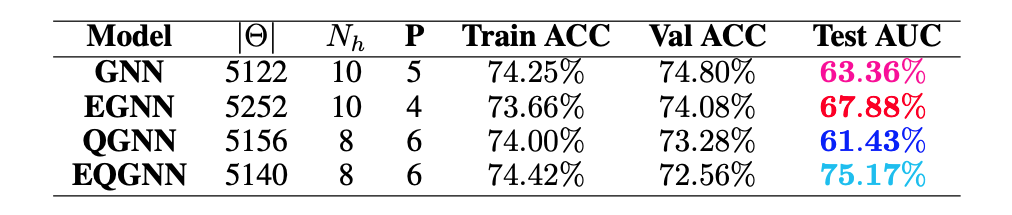
For each model, a range of total parameters were tested, however, the overall comparison test was done using the largest optimal number of total parameters for each network. A feed forward NN was used to reduce each network’s graph layered output to a binary one followed by the softmax activation function to obtain the logits in the classical case and the norm of the complex values to obtain the logits in the quantum case. Each model trained over \(20\) epochs with the Adam optimizer consisting of a learning rate of \(\eta = 10^{-3}\) and a cross-entropy loss function. The classical networks trained with a batch size of \(64\) and the quantum networks with a batch size of one due to the limited capabilities of broadcasting unitary operators in the quantum APIs. The best model weights were saved when the validation AUC, or area under the curve of the true positive rate (TPR) as a function of the false positive rate (FPR), was maximized after epoch \(15\). The results of the training for the largest optimal total number of parameters \(\Theta \approx 5100\) can be seen in the figures below.
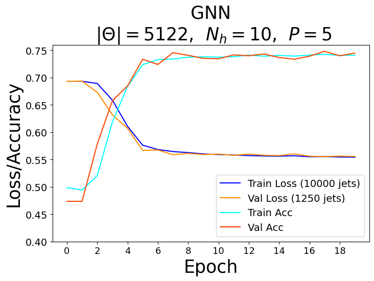
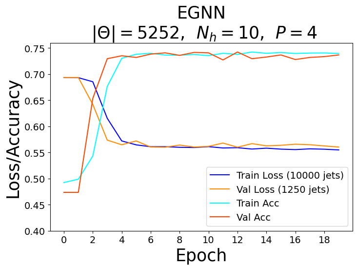
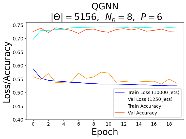
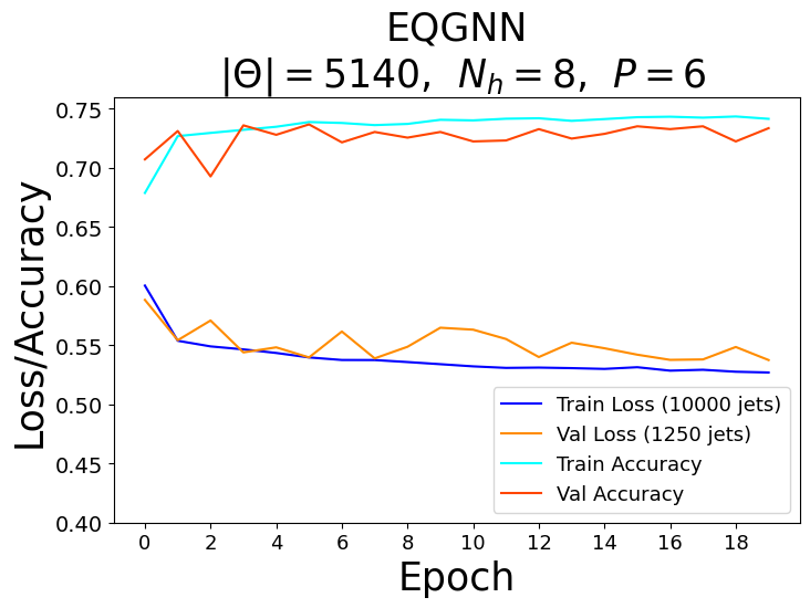
Recall that for each model, we vary the number of hidden features \(N_h\) in the \(P\) graph layers. Since we fix the number of nodes \(n_\alpha = 3\) per jet, the hidden feature number \(N_h = 2^3 = 8\) becomes fixed in the quantum case, and therefore, we also varied the parameters of the encoder \(\phi_{\psi^0 }\) and decoder NN in the quantum algorithms.
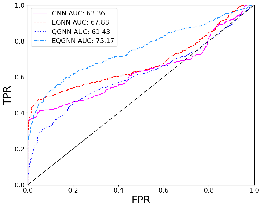
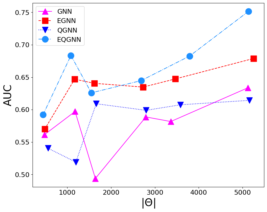
Based on the AUC scores, the EGNN outperformed both the classical and quantum GNN, however, this algortihm was outperformed by the EQGNN with a \(7.29 \%\) increase in AUC representing the strength of the EQGNN. Although the GNN outperformed the QGNN in the final parameter test by \(1.93 \%\), the QGNN performed more consistently and outperformed the GNN in the mid parameter range \(\Theta \in (1500,4000)\). Through the variation of the number of parameters, the AUC scores were recorded for each case where the number of parameters taken for each point corresponds to \(\Theta \approx \{500, 1200, 1600, 2800, 3500, 5100 \}\) as shown in the right panel of the figure above.
Conclusion
Through several computational experiments, the quantum GNNs seem to exhibit enhanced classifier performance over their classical GNN counterparts based on the best test AUC scores produced after the training of the models while relying on a similar number of parameters, hyperparameters, and model structures. These results seem promising for the quantum advantage over classical models. Despite this result, the quantum algorithms take over $100$ times as long to train than the classical networks. This may be attributed to the limited capabilities in the quantum APIs, where the inability to train with broadcastable unitary operators forced the quantum models to take in a batch size of one, or train on a single graph at a time.
The hyperparameters of the models should continue to be fine-tuned for an improved training performance. The action of the equivariance in the EGNN and EQGNN could be further explored and developed. This is especially true in the quantum case where more general permutation and SU(2) equivariance have been explored Expanding the flexibility of the networks to an arbitrary number of nodes per graph should also offer increased robustness, however, this may continue to pose challenges in the quantum case due to the current limited flexibility of quantum software. A variety of different forms of the networks can also be explored, such as introducing attention components and altering the structure of the quantum graph layers to achieve enhanced performance of both classical and quantum GNNs. In particular, one can further parameterize the quantum graph layer structure to better align with the total number of parameters used in the classical structures.
Software, Data, and Code
Software and packages used in the making of this project include the python programming language, jupyter notebooks, github, University of Florida’s HiPerGator supercomputer in a partnership with NVIDIA, Numpy, PyTorch, Pennylane. HiPerGator has the capacity to run on up to 8 GPUs and 8 CPUs with 64 GB RAM over 72 hours. Thus far, Mattermost and Medium have been used for connectivity and blogging.
The dataset used here is the Pythia8 Quark and Gluon Jets for Energy Flow dataset
The code can be found at GitHub-royforestano.